Moments Problem. Finding lexicographycally best CDF from a class M of CDF with given n moments.
The class M of CDF on [a, b] should be chosen from the list of classes available in Menu. The Monotone Calculator reconstructs a cumulative distribution function "σ" from the class M by its first n moments:
∫abt1dσ(t) = c1,
...
∫abtndσ(t) = cn,
(1.1)
where σ ∈ M.
The Calculator can do it for n ≤ 10, the class of CDF from the list of classes presented in Menu, any set of moments c1, ..., cn and any finite interval [a, b]. If there is no such CDFs, we find the one with maximal possible number of coinciding first moments. It is unique. If there are many CDF with these moments we present a unique one with maximal (n + 1)st moment and a unique one with minimal (n + 1)st moment.
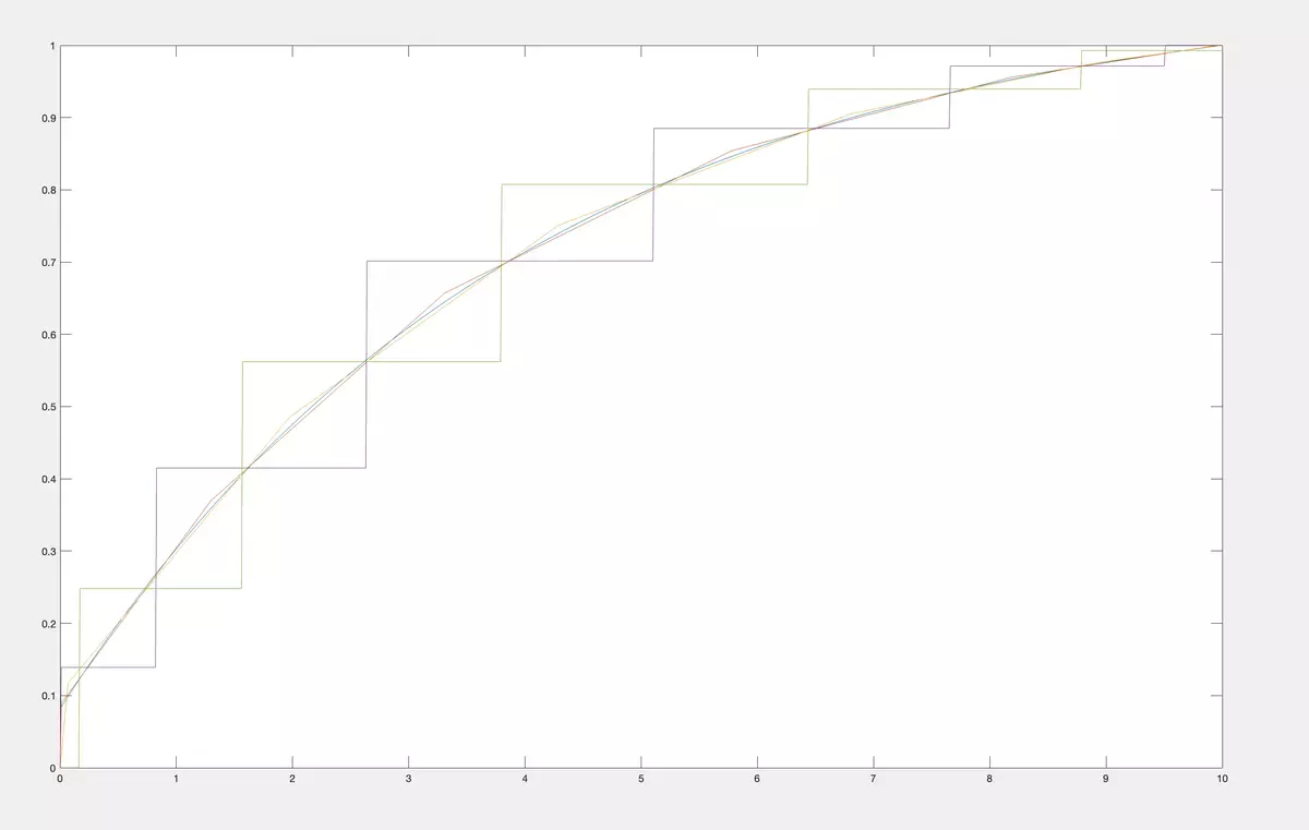
In the examples below, we took a CDF from a class M2 of concave CDF on [0, 10] (in blue).
We calculated its first 10 moments (c1, ..., c10).
For these moments we reconstruct the CDF from the class M1 of all CDF on [0, 10]. Naturally, there are many such CDFs. So, we choose the ones that maximize and correspondingly minimize the 11-th moments. Their plots are in the figure below.
Then we reconstruct the CDF from the class of M2 of concave CDF on [0, 10]. Their plots are in the figure below.
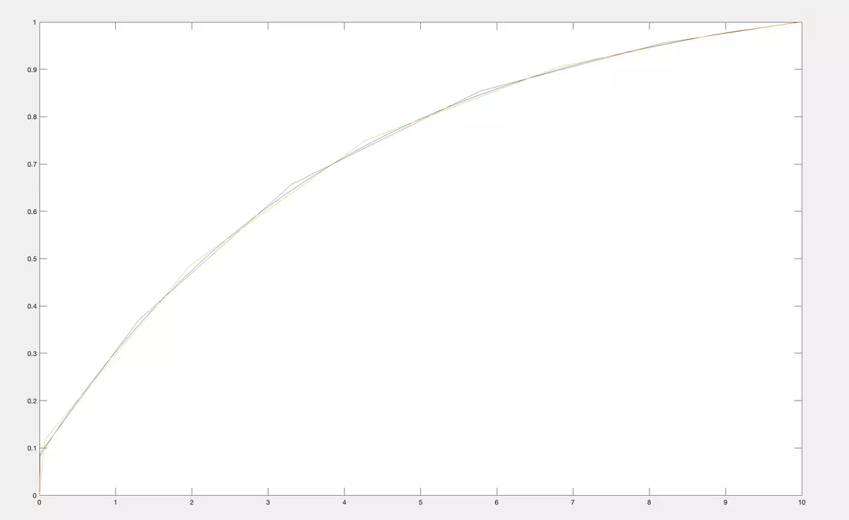
Let us compare it in the same figure.
As you see, having qualitative information about CDF allows much much better reconstruction.
Moments Problem. Finding the best CDF from a class of CDF in minimax sense.
We solve the same problem as in the previous paragraph, but here if there is no CDF satisfying moments equations we look for a CDF that minimizes
max{ |∫abt1dσ(t) - c1|, ..., |∫abtndσ(t) - cn| }.
Here, we have additional assumption: a > 0.
Chebyshev Inequality. Finding bounds of CDF at a fixed point.
If there are many CDFs from the class M having fixed moments c1, ..., cn,, we will find exact upper and lower limits of their values at a fixed point x ∈ [a, b]. We plot it for all x ∈ [a, b]. Thus, all CDFs from the class M with moments c1, ..., cn are confined between the exact upper and lower bounds.
In the examples below, we took the same CDF from a class M2 of concave CDF on [0, 10] (in blue) as in the previous paragraph. We calculated its first 10 moments (c1, ..., c10).
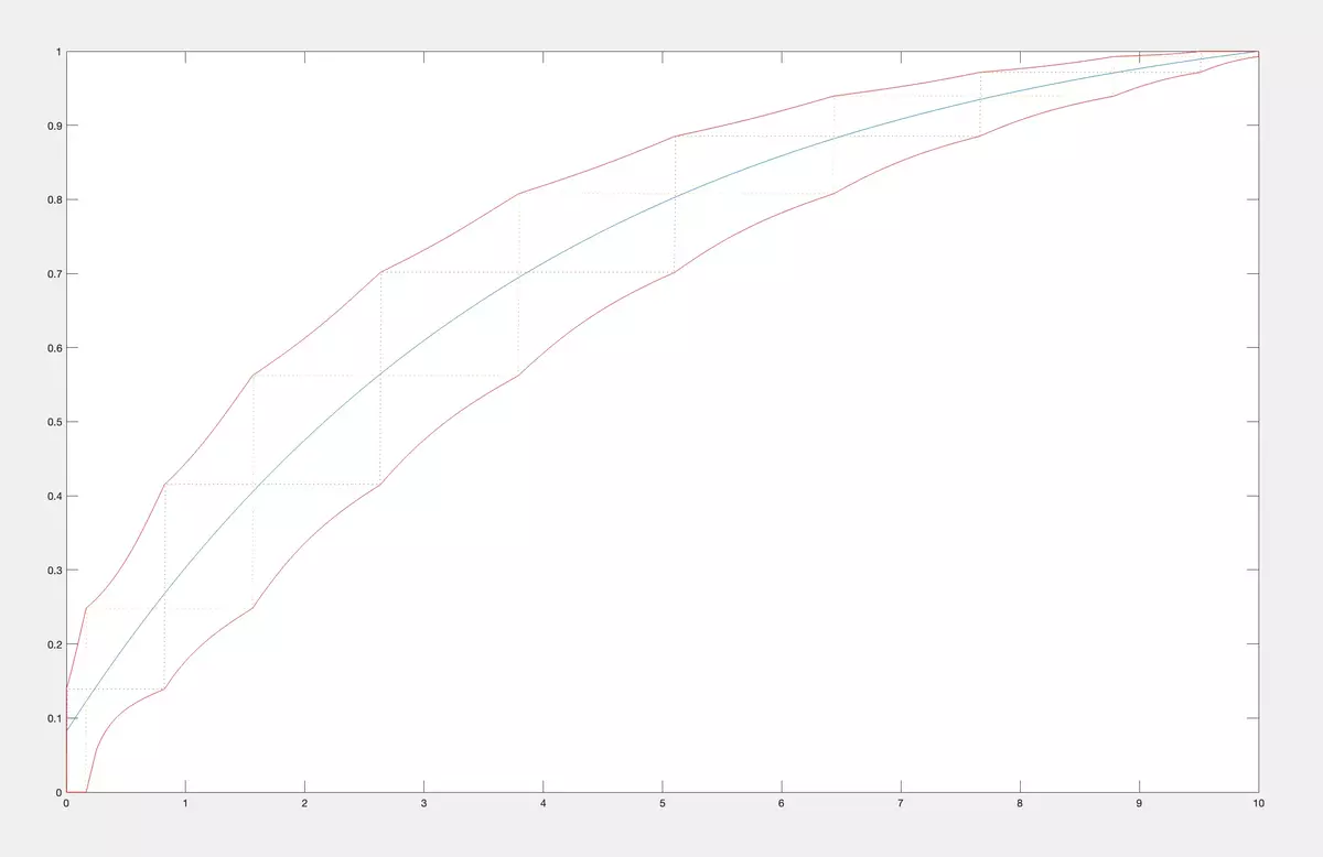
In the figure below we calculate and plot the exact upper and lower bounds for values of CDFs for the class M1 of all CDF on [0, 10] having first 10 moments equal to (c1, ..., c10).
Then we plot bounds for CDFs from the class of M2 of concave CDF on [0, 10] having first 10 moments equal to (c1, ..., c10). The exact upper and lower bounds are in the figure below.
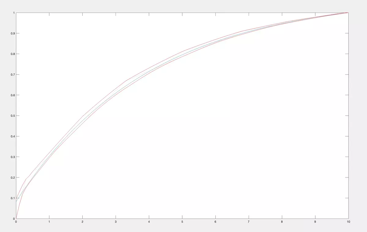
Now, let us compare them in the same figure.
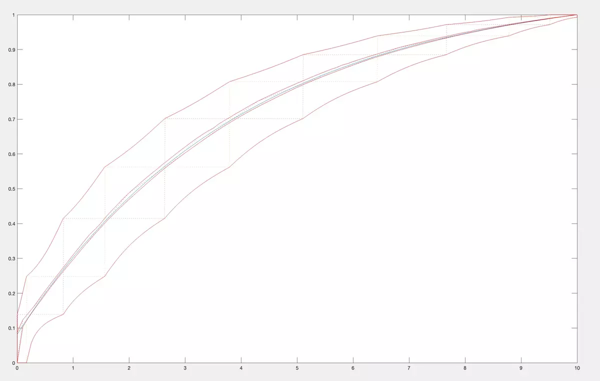
As you see, having qualitative information about CDF makes the bounds more tight.
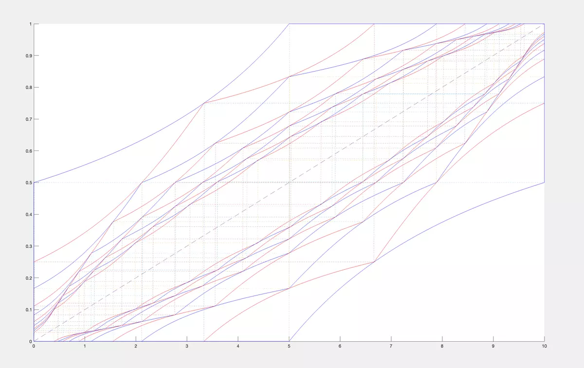
Let us consider another example to see how the bounds change when we increase n from 1 to 10. We calculate first 10 moments of a uniform CDF on [0, 10] and denote them as (c1, ..., c10). Then we calculate the bounds for values at point x of CDF from the class M1 of all CDF having fixed moments (c1, ..., cn) for n = 1, then n = 2, up to n = 10. We alternate colors blue, red,blue, red when moving from 1 to 10.
Chebyshev Plus Inequality.
We fix points x and y such that a ≤ x < y ≤ b. We will find here exact lower and upper bounds for the difference σ(y) − σ(x) for all CDF σ from the class M having fixed moments c1, ..., c. Thus, our task is to find the bounds for the probability that random variable takes values between x and y if we know that its CDF is from the class M and its moments equal to c1, ..., cn.