Monotone Calculator. Menu. Manual.
Karen Tatalyan
Fund ”monotoneprogramming.com”
tatalyan@monotoneprogramming.com
Chapter 0
Introduction
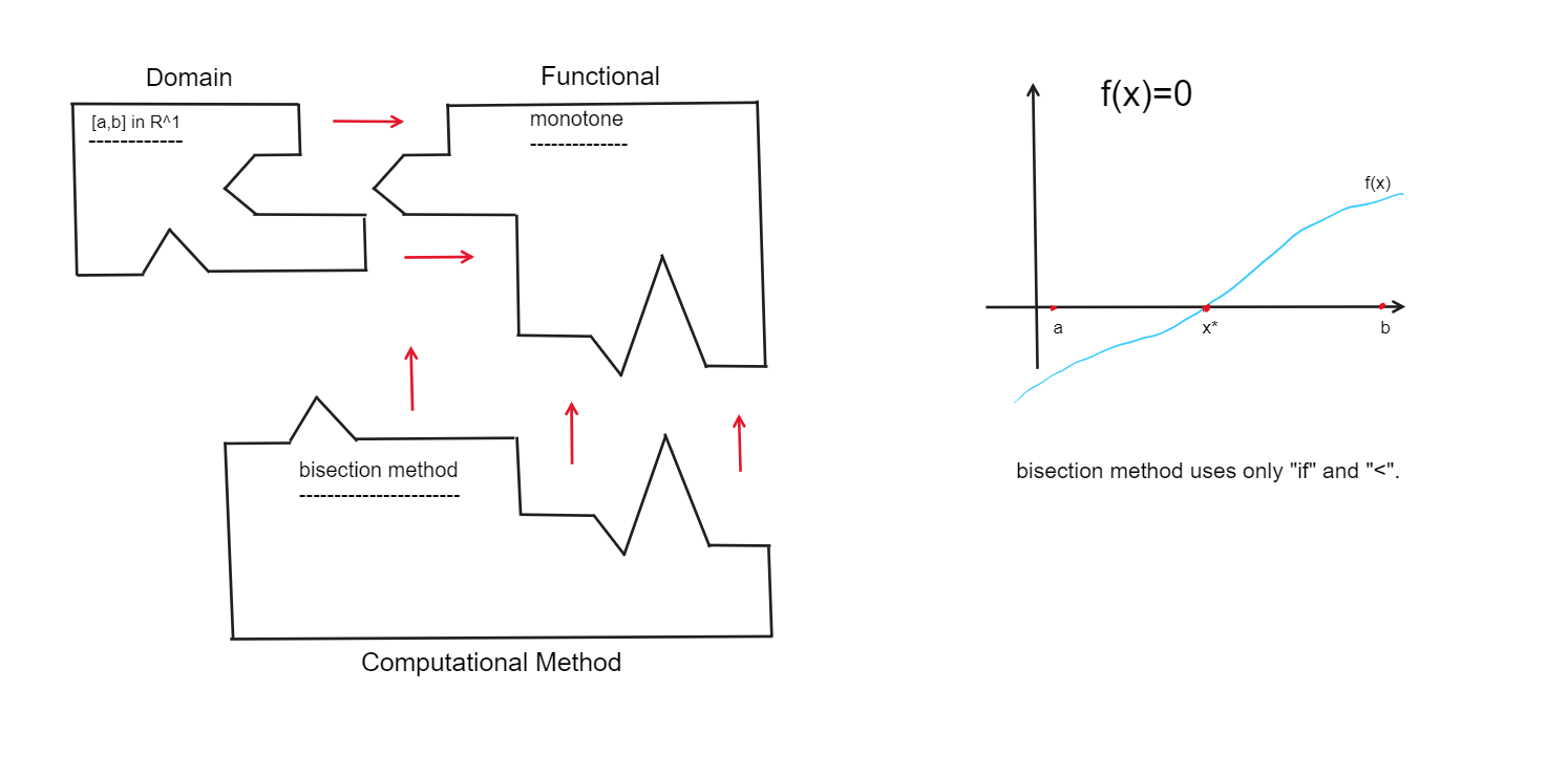
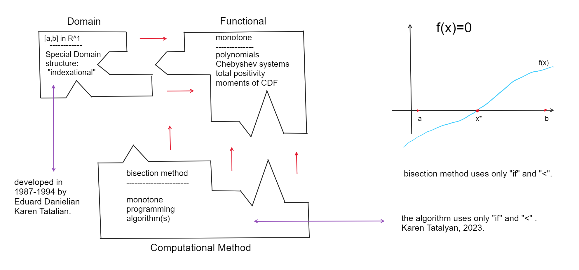
We introduce here Monotone Calculator. What it calculates and How? The What. It allows to solve a list of very practical problems in Probability and Statistics, Optimal Control, Polynomials. To our knowledge majority of these problems were not calculable before. They are described in section Monotone Calculator. Particularly, for cumulative distribution functions on a finite interval, Monotone Calculator solves a set of minimization problems with up to 10moments. At present Monotone Calculator solves a dozen of problems. Its number will reach a hundred in a year. We project a thousand quite practical problems solution in five year perspective. What unites all these at first sight quite unconnected or irrelevant problems? They have similar internal structure that is invisible at first sight. Therefore, to solve them we can apply the same method. The same How. The How. All functionalities in Monotone Calculator work with one basic algorithm we called Monotone Programming. It is an original method based exclusively on the notion of monotonicity. It does not use any of XVI-XXI centuries math. It could be used in Ancient Greece if they had calculators. Actually, even “plus”, “minus”, “multiplication” and “division” operations are not used. The method is using only “if”s and “<”s. Do we have something similar in computational mathematics? Sure. It is so called bisection method. Let us describe it. We should solve the equation
f(x) = 0,where functionf(x) is a monotone (increasing) function. What we do? We take any initialx. Then iff(x)< 0 ,we go right and if not we go left. Then we repeat. Thus, we reach a unique solution with the exactness we wish.
I remember, when I was a student and was introduced to bisection method during the course of Computational Methods I was disappointed that it does not have any continuation. Here, by mere existence of Monotone Calculator we show that such extensions exist and we successfully apply them to solve a range of problems in Probability and Statistics, Optimal Control and Polynomials. However, in spite of its “simplicity” and theoretical possibility to be discovered even in ancient Greece, to suspect that such sort of extension of bisection method exists a mathematician should have a very specific set of knowledge that takes its roots from Total Positivity up to… Algebraic Topology. I consider myself not an author but a discoverer of the method, or a group of methods that I called Monotone Programming. I still do not understand fully why does it work. I managed to write the code only because at some point I understood that it exists. Then, like an archeologist, I just unearthed it.
Monotone Calculator has a commercial value. We now in a process to evaluate it. It will take some time. That is why here we will not present the codes but will demonstrate the capacity of Monotone Calculator, the added value it brings to Statistics and Probability and some new results. There are submenues ”Menu Probability”, ”Menu Statistics”, ”Menu Polynomials”, ”Menu Optimal Control” and ”Menu Others” for other problems that does not fall into first four menues.
Chapter 1
Menu Probability:
1.1 Classes of cumulative distribution functions (CDF).
1.1.1 Classes of CDF on[a,∞]
- Class of all CDF on[a,∞].
1.1.2 Classes of CDF on finite[a, b]
There is a list of classesMof CDF on [a,b] with which we work.
- ClassM 1 of all CDF.
- ClassM 2 of concave CDF.
- ClassM 3 of CDF confined between fixed upper CDF and fixed lower CDF. A class of CDF whose plots pass through fixed sets of points could be presented as being confined between two CDFs.
- ClassM 4 of CDF with bounded densities.
- ClassM 5 of convex CDF.
- ClassM 6 of Increasing Hazard Rate CDF (”aging” like humans).
- ClassM 7 of Decreasing Hazard Rate CDF (”becoming younger with age” like some electronics).
- ClassM 8 of Increasing in Average Hazard Rate CDF.
- ClassM 9 of Decreasing in Average Hazard Rate CDF.
- Class of Bell Shaped CDF.
- Class of First Convex and then Concave CDF (densities first increasing, then decreasing).
1.2 Extremal problems with fixed moment on classes of CDF.
1.2.1 Moments Problem. Finding lexicographycally best CDF from a
classMof CDF with givennmoments.
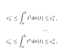
The classMof CDF on [a,b] should be chosen from the list of classes available in Menu. The Monotone Calculator reconstructs a cumulative distribution functionσfrom the classMby its firstnmoments:
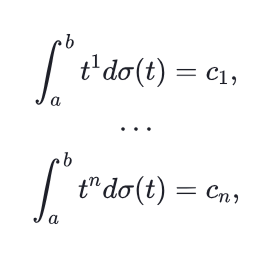
(1.1)
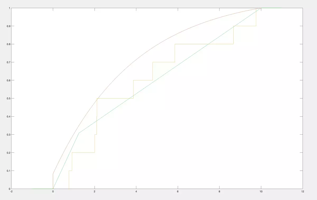
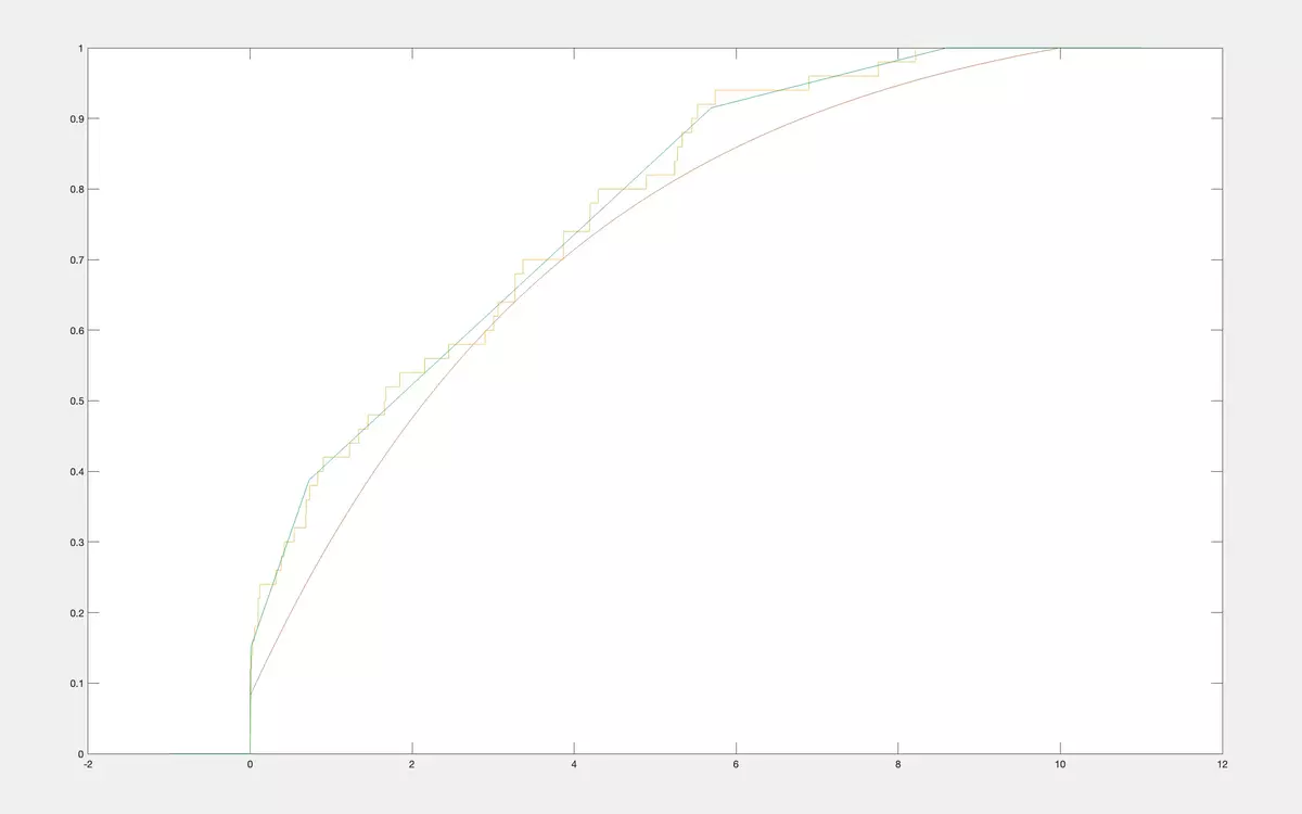
whereσ∈M. The Calculator can do it forn≤10, the class of CDF from the list of classes presented in Menu, any set of momentsc 1 ,…,cnand any finite interval [a,b]. If there is no such CDFs, we find the one with maximal possible number of coinciding first moments. It is unique. If there are many CDF with these moments we present a unique one with maximal (n+ 1)st moment and a unique one with minimal (n+ 1)st moment. In the examples below, we took a CDF from a classM 2 of concave CDF on [0,10] (in blue). We calculated its first 10 moments (c 1 ,…,c 10 ). For these moments we reconstruct the CDF from the classM 1 of all CDF on [0,10]. Naturally, there are many such CDFs. So, we choose the ones that maximize and correspondingly minimize the 11-th moments. Their plots are in the figure below.
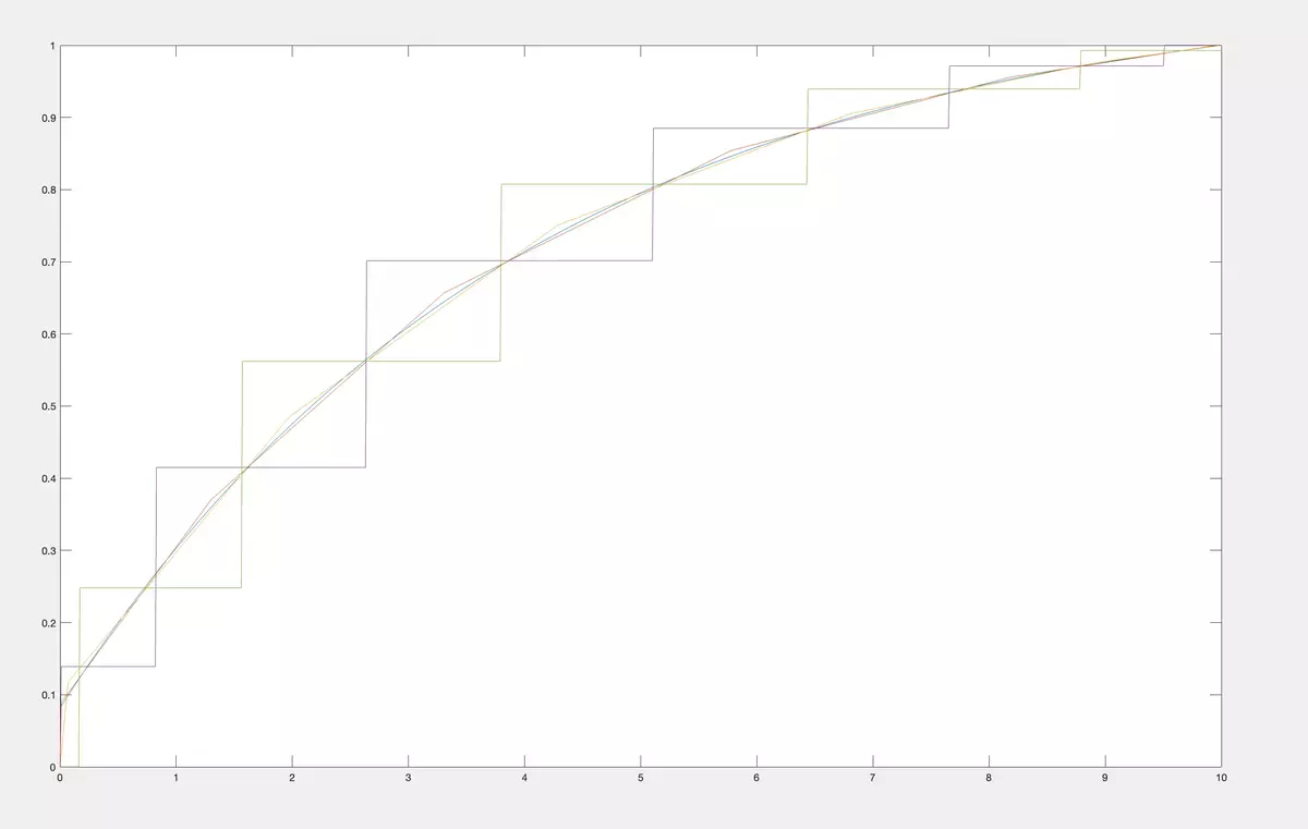
Then we reconstruct the CDF from the class ofM 2 of concave CDF on [0,10]. Their plots are in the figure below.
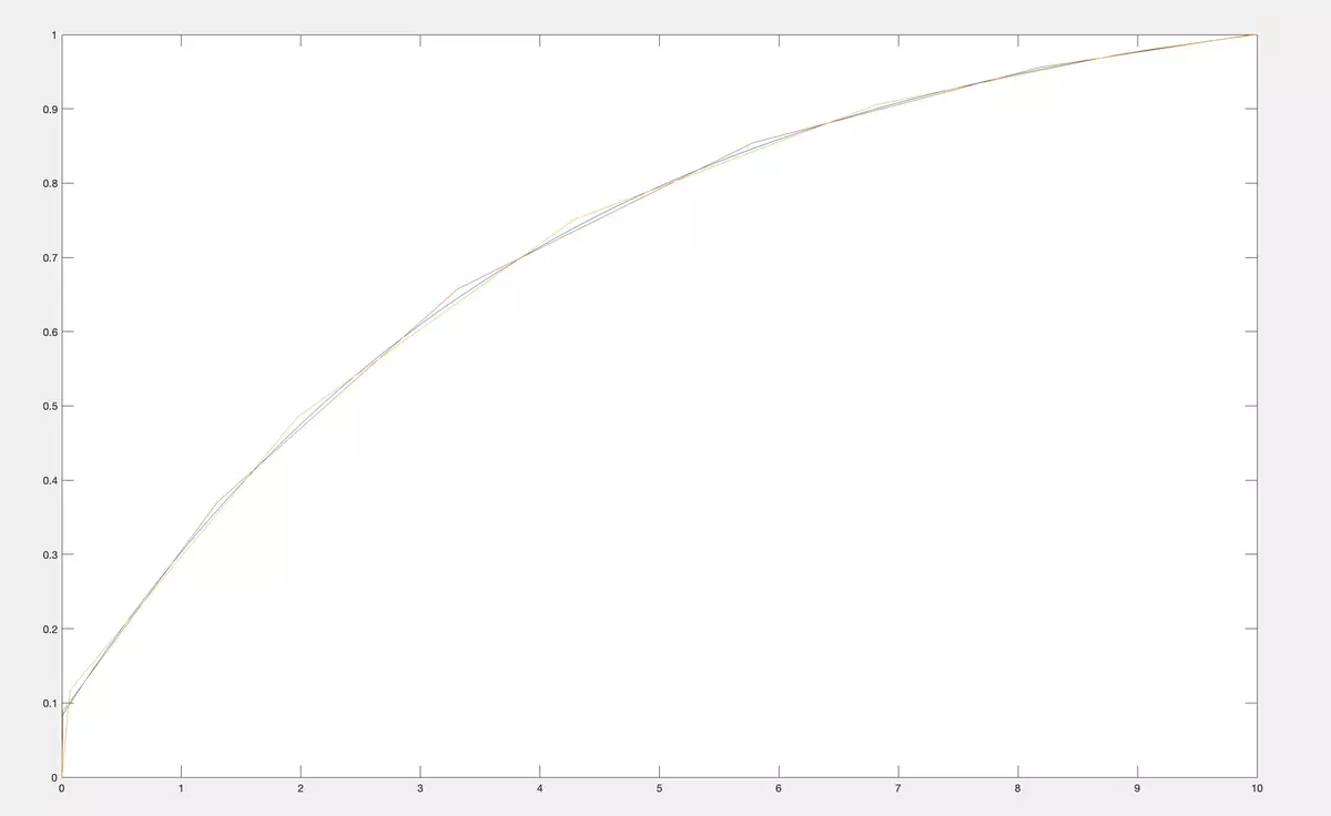
Let us compare it in the same figure.
As you see, having qualitative information about CDF allows much much better reconstruction.
1.2.2 Moments Problem. Finding the best CDF from a class of CDF in
minimax sense.
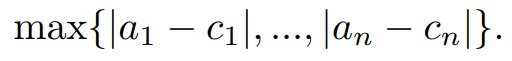
We solve the same problem as in the previous paragraph, but here if there is no CDF satisfying moments equations we look for a CDF that minimizes
Here, we have additional assumption:a >0.
1.2.3 Chebyshev Inequality. Finding bounds of CDF at a fixed point
x∈[a, b].
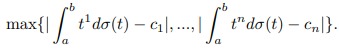
If there are many CDFs from the classMhaving fixed momentsc 1 ,…,cn, we will find exact upper and lower limits of their values at a fixed pointx∈[a,b]. We plot it for allx∈[a,b]. Thus, all CDFs from the classMwith momentsc 1 ,…,cnare confined between the exact upper and lower bounds. In the examples below, we took the same CDF from a classM 2 of concave CDF on [0,10] (in blue) as in the previous paragraph. We calculated its first 10 moments (c 1 ,…,c 10 ). In the figure below we calculate and plot the exact upper and lower bounds for values of CDFs for the classM 1 of all CDF on [0,10] having first 10 moments equal to (c 1 ,…,c 10 ).
Then we plot bounds for CDFs from the class ofM 2 of concave CDF on [0,10] having first 10 mo- ments equal to (c 1 ,…,c 10 ). The exact upper and lower bounds are in the figure below.
Now, let us compare them in the same figure.
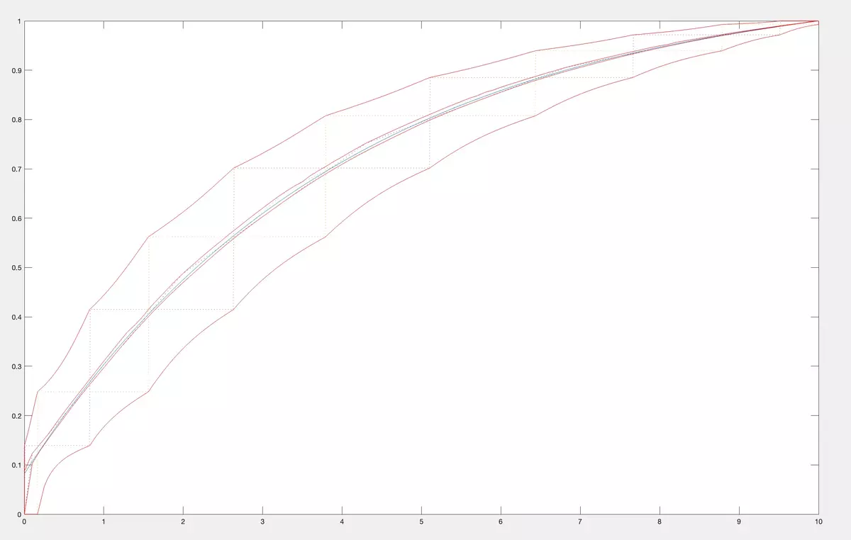
As you see, having qualitative information about CDF makes the bounds more tight.
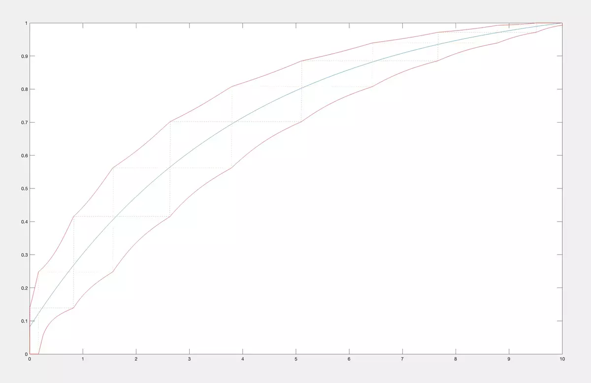
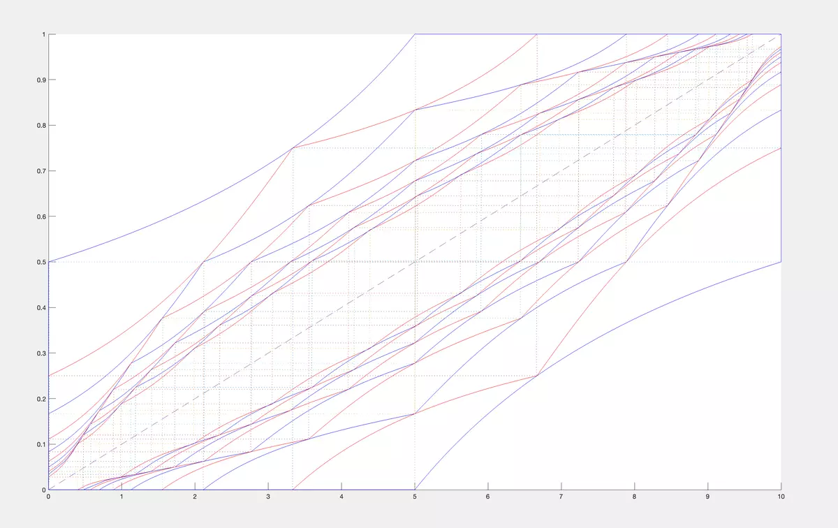
Let us consider another example to see how the bounds change when we increasenfrom 1 to
- We calculate first 10 moments of a uniform CDF on [0,10] and denote them as (c 1 ,…,c 10 ). Then we calculate the bounds for values at pointxof CDF from the classM 1 of all CDF having fixed moments (c 1 ,…,cn) forn= 1, thenn= 2, up ton= 10. We alternate colors blue, red,blue, red when moving from 1 to 10.
1.2.4 Chebyshev Plus Inequality.
We fix points x and y such that a ≤ x < y ≤ b. We will find here exact lower and upper bounds for the difference σ(y) − σ(x) for all CDF σ from the class M having fixed moments c1, ..., cn. Thus, our task is to find the bounds for the probability that random variable takes values between x and y if we know that its CDF is from the class M and its moments equal to c1, ..., cn.
1.3 Extremal problems with moments from parallelepiped.
on classes of CDF.
The same problems as in previous section but instead of assuming that moments are fixed we assume that moments are from an interval.
(1.2)
where σ ∈ M.
Chapter 2
Menu Statistics.
2.1 Classes of cumulative distribution functions (CDF).
We work with the same list of classes of CDF as in Menu Probability. Exception is the class of all CDF for which the Moment Method is a tautology. Indeed, the empiric CDF are naturally from the classof all CDF.
2.2 Method of Moments.
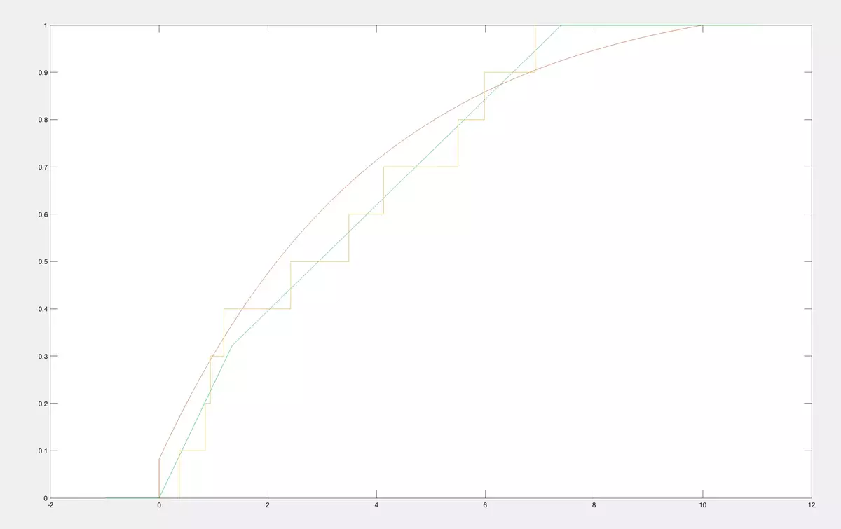
As we are able to reconstruct CDF from a class by its moments for anyc 1 ,…,cn, we can do it for firstnempirical moments of a sample and, therefore, we can effectively apply the moments method to estimate the CDF from a nonparametric class. It is not a staircase empirical CDF but a unique CDF from a nonparametric class that have maximal possible first moments coinciding with the empirical ones. Below, we bring examples. As an original CDF we take the same CDF from the classM 2 of concave CDF on [0,10] as in previous examples. Then we do simulations and get correspondingly 7 realizations of the random variable.
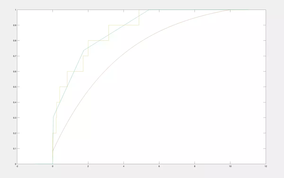
then 10 realizations twice
then 50 realizations three times
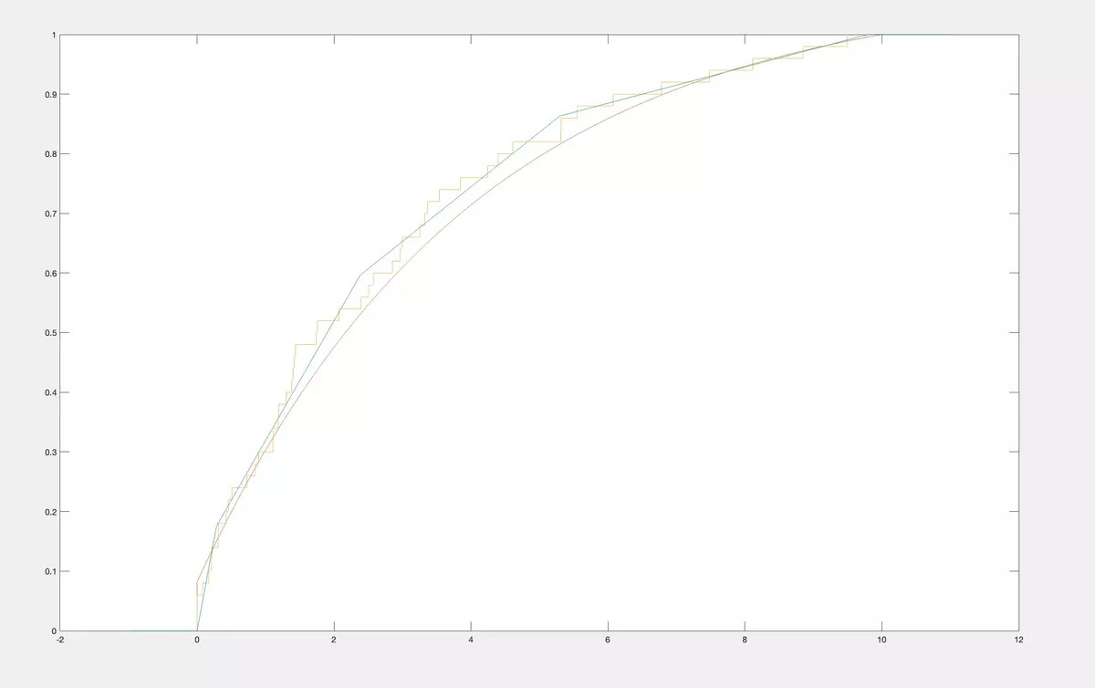
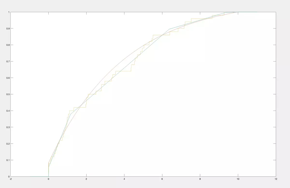
As you see, instead of empirical CDF we construct CDF from the classM 2 of concave CDF on [0,10] having best approximation to empirical moments. Naturally, it is much more practical to work with CDF from the class than with empirical CDF. Like empiric CDFs our CDFs also tend to the original CDF whenntends to infinity.
Chapter 3
Menu Polynomials.
3.1 Minimax Approximation.
Given a polynomial

Among polynomials

havingnreal positive roots find one whose coefficienfs are the closest to (c 1 ,…,cn) and calculate its roots. Saying the closest we understand coefficients that minimize
Slight modification of it is also sovable.: Among polynomials

havingnreal roots lying in [a,b], where 0≤a < b <∞, find a polynomial whose coefficienfs are the closest to (c 1 ,…,cn) and calculate its roots.
Routine: TrueAlternanceDiscreteSimplexFinale.
3.2 Minimax Approximation.*
Let us consider system of functions
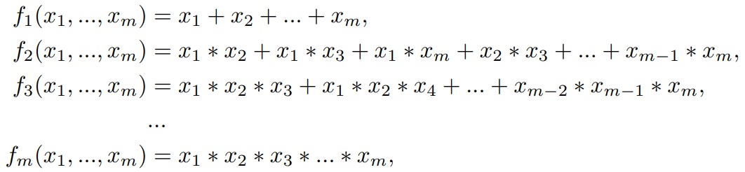
(3.1)
defined onM={(x 1 ,...,xm) :∞> b≥x 1 ≥x 2 ≥...xm≥a≥ 0 }, whereaandbare fixed.
For fixedn(n≤m) and (c 1 ,...,cn) solve a system of equations
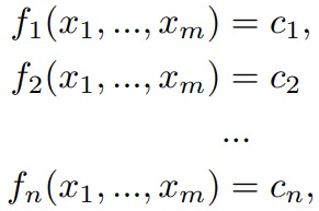
(3.2)
If solution does not exist find (x∗ 1 ,…,x∗n) fromMthat minimizes

Routine: TrueAlternanceDiscreteSimplexatob.
3.3 Lexicographical Approximation.
Given a polynomial

Among polynomials

havingnreal roots find one whose coefficienfs are the closest to (c 1 ,…,cn) and find its roots. Slight modification of it is also sovable.: Among polynomials

havingnreal roots lying in [a,b], where∞ ≤a < b <∞, find a polynomial whose coefficienfs are the closest to (c 1 ,…,cn) and calculate its roots. Saying the closest we understand lexicographycal way, i.e. that the maximal number of first coefficients coinside.
Routine: LexicoDiscreteSimplexInProcess.
3.4 Lexicographical Approximation.*
Let us consider system of functions
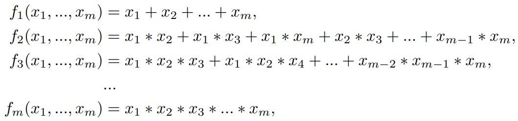
(3.3)
defined on M={(x 1 ,...,xm) : ∞> b ≥ x 1 ≥ x 2 ≥...xm ≥ a ≥ 0}, whereaandbare fixed.
For fixedn(n≤m) and (c 1 ,...,cn) solve a system of equations
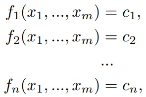
(3.4)
If solution does not exist find (x∗ 1 ,…,x∗n) fromMsuch that (f 1 (x∗ 1 ,…,x∗m),…,fn(x∗ 1 ,…,x∗m)) is lexicographically closest to (c 1 ,…,cn), i.e. the maximal number of first coefficients coinside.
Routine: LexicoDiscreteSimplexInProcess.